Development
The first half of the project was an effort to understand the functioning of Scilab and contributing something essential at the same time. This was done by creating a standalone machine learning toolbox for Scilab with all codes written in pure Scilab. This included undestanding the underlying concepts of different machine learning techniques and also, how Scilab function
In this blog post, I would guide you through the ups and downs, the highs and lows of what came to be known as Machine_Learning to all the users of Atoms. All of the updates and code can be veiwed on the github sub-repository.
Work progress
The daily work updates for this toolbox as well as the other toolbox (cloud based) are available on the scilab-wiki page.
Usage
The usage would be explained via a series of screenshots. These are a postcursor to instlalling the toolbox and loading it. We would view one preprocessing (1-hot-encode) and one algorithm (affinity clustering) for the demo.
1 hot encoding
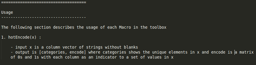
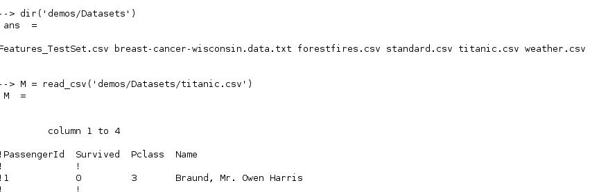
This can be viewed in the readme file for the toolbox. Thus we prepare a vector of strings from one of our datasets for the demo and then remove blanks. Then we proceed with the usage of the toolbox with the commands hotEncode. Just for the sake of the demo, we list out the datasets in the demos for the toolbox and then read the titanic dataset using the read_csv command
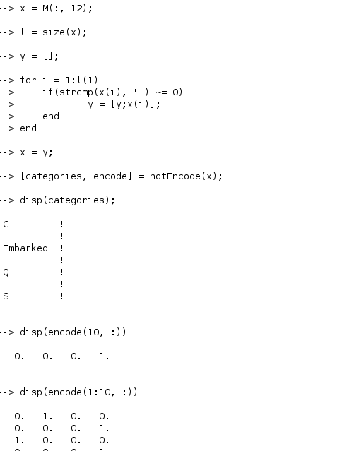
Then we select column 12. We remove any blank fields from the column. Then we run the hotEncode command which according to the readme returns the categories and encode variables. The category variable represents the different classes in the column and encode gives us the required encoding.
Affinity cluster
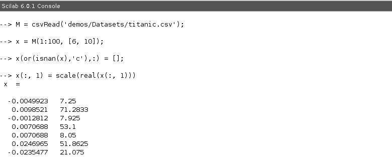
We now read the dataset as shown earlier and both the columns are then scaled (it is known to give better results though , not necessary to do it).
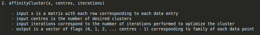
We can see from the readme.txt file that this requires three inputs - the data, the number of proposed centres and the number of iterations for convergence. We use 3 centres and 4 iterations
We use the function affinityCluster(x, 3, 4) which results in a set for flags. We run unique/tabul flags to see the distribution of assignment.
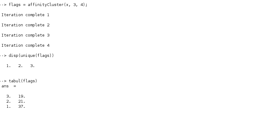
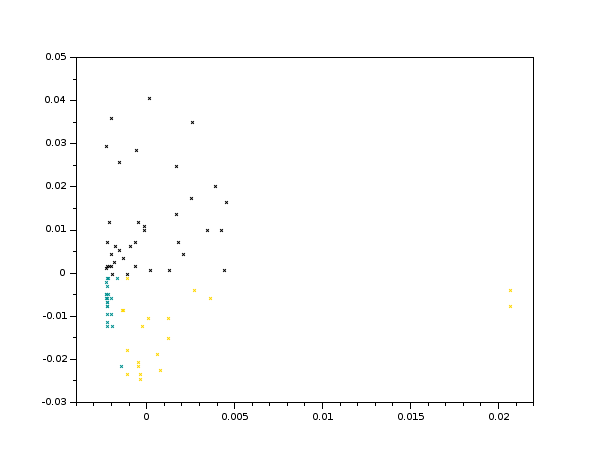
We can then plot these flag values with our original data to get the following plot
Testing
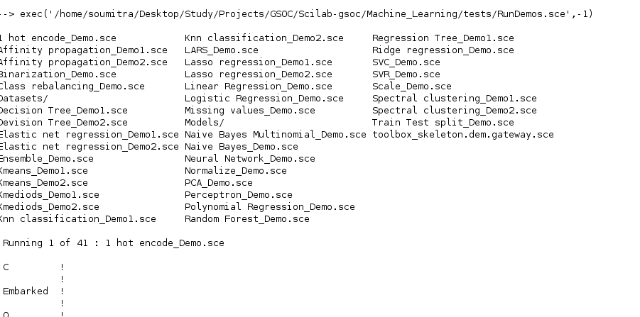
A seperate file for testing each of the given algorithms was written. To test them out yourself you can wander into the tests directory in the toolbox to the following view.

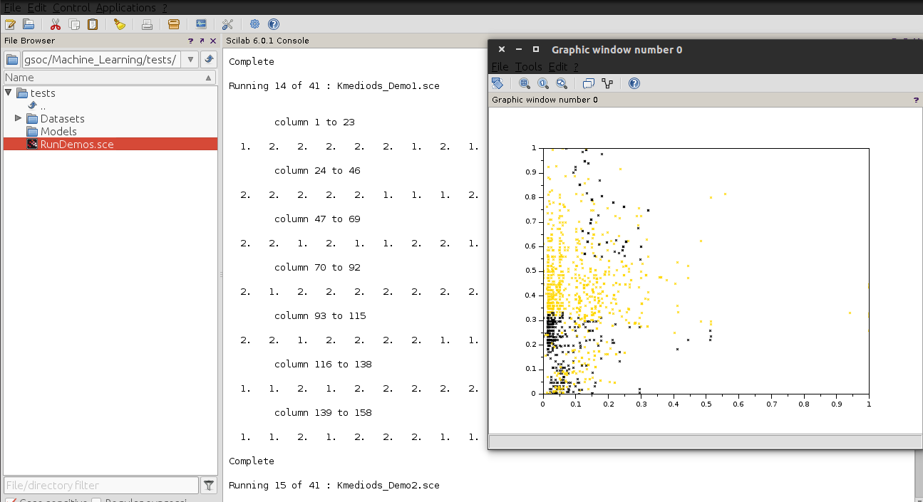
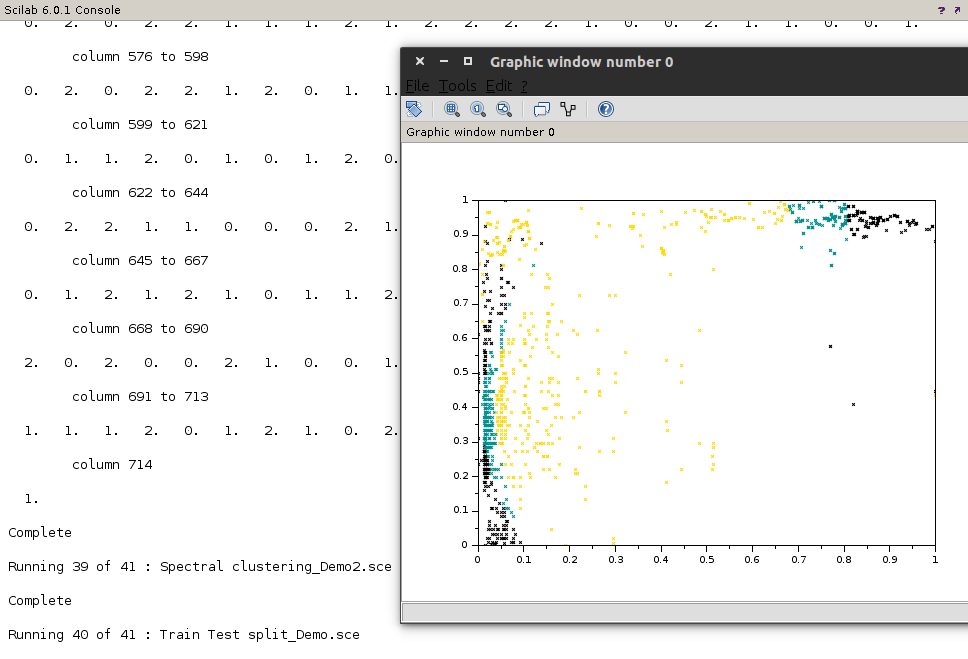
One can run the RunDemos.sce using Scilab. It proceeds to run all the macros in your demos directory (which boils down to 41 machine learning test over all the macros) and keeps you updated ![]() . Here are some of the highlights
. Here are some of the highlights